Abstract
Background. Economic preparedness for African swine fever (ASF) requires an account of disruption beyond animals lost: market access, farm liquidity, processing bottlenecks and the distribution of recovery costs. Objectives. This paper asks how trade recognition changes market incidence, how losses differ among pig enterprises, when extra processing capacity reduces backlog costs, and under what conditions compartment investment covers its costs. Data and methods. A 2025 UK pigmeat balance calibrates a deterministic partial-equilibrium model. Separate illustrative enterprise budgets, weekly incremental cash accounts, a finite-horizon processing programme and a discounted investment appraisal address different decision boundaries. These modules are complementary and are not added into a national total.
Results. In the domestic-pig scenarios, moving from no recognition to 80% recognition changes the price response from -6.95% to 0.39% and reduces the modelled producer-surplus loss from £103.08m to £37.08m over 26 weeks. That improvement is not a gain of the same size in national welfare. Farm examples show that peak cash needs can substantially exceed economic loss. The processing example avoids £408,678 relative to unchanged capacity, conditional on the assumed capacity being feasible. At the compartment defaults, NPV is £-11.32m and the benefit–cost ratio is 0.15. Interpretation. These are conditional economic calculations, not outbreak forecasts or representative-farm estimates. The contribution is a transparent set of accounting boundaries, thresholds and reproducible tests for preparedness decisions.
Keywords: African swine fever; pig economics; indirect costs; partial equilibrium; cash flow; regionalisation; compartmentalisation; recovery; United Kingdom.
1. Background and introduction
An ASF emergency would affect businesses through several channels with different clocks. Animals and productive assets can be lost immediately. Marketing interruptions can withhold cash before a loss is realised. Trade restrictions can change prices across businesses with no disease on their premises. Recovery of output, breeding capacity, liquidity and market access can occur at different times. A study that reports only animals removed or a single national cost cannot show which instrument addresses which problem.
The analytical starting point is stakeholder and cost identification. Savioli et al. (2022), including co-author Bouda Vosough Ahmadi, combined regulatory review and stakeholder evidence for a hypothetical Swiss outbreak. Their catalogue of 104 measures and impacts across 14 categories demonstrates why an indirect-cost register is needed before choosing what to monetise. Here that approach informs an explicit register of affected parties, cost mechanisms, model coverage and outstanding evidence. Swiss monetary values and regulatory assumptions are not transferred to the UK.
Shared logistics also matter. Porphyre et al. (2020) studied the British pig sector using historical movement and haulage connections. That study supports including shared transport services in an economic continuity assessment. It does not define the four scenarios in this paper, provide current network data, or calibrate the assumed duration, output reduction or recognition rate. Treating it as the source of those numerical assumptions would overstate its role.
Recent work provides useful comparisons with different boundaries. Gren et al. (2024) examined Swedish response costs, including indirect effects outside conventional farm budgets. Helgesen and Barratt’s EPIC brief examines price and revenue persistence after disease freedom across linked commodities. Shakil et al. (2025) develops a vertically integrated partial-equilibrium livestock approach in another country and sector. Together these studies motivate a broader research agenda; the present application implements a smaller set of transparent economic mechanisms and identifies the missing links.
1.1 Objectives and contribution
The five objectives are to compare explicit trade/output counterfactuals; separate incidence across breeder, grower, finisher and integrated businesses; distinguish resource loss, transfers and liquidity; examine recovery and investment thresholds; and publish enough code, assumptions and numerical results to reproduce the analysis. The paper is an independent working analysis. It is not an estimated causal effect of a realised UK outbreak, an epidemiological simulation or a fully calibrated industry appraisal.
Table 1. Decision questions, estimands and boundaries
| Decision | Modelled outcome | Excluded from that outcome |
|---|---|---|
| Trade recognition | Producer and farmgate-equivalent consumer surplus; partial-market balance | Retail and processing margins, foreign welfare, differentiated products |
| Enterprise support | Private loss and a 52-week incremental liquidity bridge | Full accounts, tax, household expenditure, pre-existing debt schedule |
| Processing recovery | Least-cost backlog schedule versus standard capacity | Breeding-herd recovery and actual movement permission |
| Compartment investment | Expected avoided private loss, NPV and recognition threshold | An official risk estimate, guaranteed access or a complete social appraisal |
2. Data, geography and evidence hierarchy
The market calibration uses one annual official balance rather than combining observations with a later forecast. Defra’s Agriculture in the United Kingdom 2025 reports home-fed pigmeat production of 937 kt, imports summing to 602 kt in the rounded table, exports of 146 kt and a 204 p/kg price proxy. Model domestic availability is the accounting identity 937 + 602 − 146 = 1,393 kt. Defra’s reported supply is 1,394 kt; the one-kt difference is retained as a rounding reconciliation rather than hidden in an artificial residual.
Table 2. Core data and interpretation (Defra, 2026a)
| Measure | 2025 value | Model role / qualification |
|---|---|---|
| Home-fed production | 937,000 tonnes | Annual domestic supply calibration |
| Imports / exports | 602,000 / 146,000 tonnes | Rounded published components; restricted product scope |
| Domestic availability | 1,393,000 tonnes | Derived identity; official reported supply 1,394,000 |
| Price proxy | £2.04/kg | Annual farmgate proxy, not a retail price |
| All pigs, June | 4.739 million | Context; not multiplied by an assumed loss per pig |
| Breeding sows / in-pig gilts | 277,000 / 39,000 | Distinct categories; 277,000 is not all female breeding stock |
| Average clean-pig carcase weight | 91 kg | Combined with price to illustrate £185.64 per marketed finisher |
The trade series covers fresh, chilled, frozen and salted/brined pigmeat on its stated bone-in-equivalent basis; it excludes offal and manufactured or preserved products. The exercise therefore does not measure the value of every pork export market. Quantities from the statistical balance are treated as commensurate in the homogeneous-market approximation. Detailed product conversion factors, unit values and destination-specific restrictions would be needed for a trade appraisal.
AHDB’s Q1 2026 release estimates full economic production cost at 192 p/kg and margin at −£3.85 per slaughter pig. This is context for financial resilience, not the source of the positive contribution margins used below: full economic margin and contribution after avoidable variable cost are different quantities. AHDB’s June 2026 outlook forecasts 1.03 million tonnes of 2026 production using a 978 kt 2025 comparator. That comparator differs from the 937 kt Defra series. The difference has not been reconciled here, so the forecast is not spliced into the calibration (AHDB, 2026a,b).
The commodity baseline is UK-wide. The cited swine-fever strategy is for Great Britain (Defra, 2026b). Northern Ireland requires separate interpretation of applicable animal-health and trading arrangements. Neither a UK aggregate market balance nor a GB policy document establishes a single operational regime for every holding. No regional output shocks are inferred from farm locations.
2.1 Observations, assumptions and model outputs
Observed statistics establish scale. Economic response parameters, loss durations and farm templates are illustrative assumptions. Model outputs follow from those inputs and equations. Published studies inform mechanism selection and the discussion; they do not convert the assumed values into estimates. A national pig-and-wild-boar map is omitted because a comparable, current UK-wide wild-boar population layer and harmonised pig geography were not verified for this release. A polished basemap alone would not resolve that evidential problem.
Table 3. Market assumption register
| Input | Default / range examined | Provenance and interpretation |
|---|---|---|
| Shock duration | 26 weeks; 13, 26, 52 | Illustrative constant economic disruption, not disease persistence |
| Domestic output shift | 0% W cases; 5% D cases; 0–20% sensitivity | Exogenous economic quantity reduction; no epidemic calibration |
| Initial export blockage | 100% | Stress assumption for included export products |
| Recognition / restricted share | 0 or 80%; restricted share 10% | Assumed eligible-market recognition and uniform regional production proxy |
| Supply / demand elasticity | 0.30 / 0.40 | Illustrative local slopes, not UK econometric estimates |
| Import / export elasticity | 1.00 / 1.00 | Illustrative trade response slopes |
| Domestic demand shift | 0% | No preference response in fixed cases; editable in application |
| Control / logistics cost | W: £5m / £2m; D: £10m / £5m | One-off resource-cost allowances; uncalibrated and not sums from an impact inventory |
3. Methods and analytical framework
3.1 Scenario definition and counterfactual
The comparator is a normal-trading baseline with the observed annual balance and no output, demand or access shock. The four cases cross an assumed initial setting with a trade-recognition response. W denotes a wild-boar-associated economic stress case with no imposed domestic production loss; D adds a 5% exogenous domestic output reduction. The labels are bookkeeping devices. They do not imply that an actual wild-boar event would leave domestic output unchanged, or that a domestic event would remove exactly 5% of production.
Table 4. Fixed scenario design
| Case | Economic starting assumption | Recognition | Specified costs |
|---|---|---|---|
| W1 | No domestic output shift; initial export blockage 100% | 0% | £7m |
| W2 | Same output and blockage as W1 | 80% of eligible access | £7m |
| D1 | Domestic output shift −5%; initial export blockage 100% | 0% | £15m |
| D2 | Same output and blockage as D1 | 80% of eligible access | £15m |
All four hold duration at 26 weeks, the restricted production share at 10%, and the same market slopes. The W1–W2 and D1–D2 comparisons isolate recognition within a family. Comparing W with D also changes resource allowances, so it is not a pure production-shock contrast. The four cases have no probability weights. The 10% restricted share is used as a proxy for excluded exportable output under uniform exposure; concentration of export-oriented businesses would require a different weight.
3.2 Market clearing and surplus accounting
Let S₀, M₀ and X₀ be baseline annual production, imports and exports, D₀ = S₀ + M₀ − X₀, and r = p/p₀. Let l be the fractional output reduction, d the demand reduction, b the initially blocked export share, a recognition and z the restricted share. The effective blocked fraction is B = b[1 − a(1 − z)]. At 80% recognition and 10% restricted share, B is 28%, not 20%.
S(r) = S₀(1−l) max{0, 1+εs(r−1)}
D(r) = D₀(1−d) max{0, 1−εd(r−1)}
M(r) = M₀ max{0, 1+εm(r−1)}
X(r) = X₀(1−B) max{0, 1−εx(r−1)}
Market clearing: S(r)+M(r) = D(r)+X(r)
The code solves the non-negative linear schedules by bisection. Annual quantities are converted from tonnes to kilograms before monetary integration. Producer surplus is revenue less the integral of inverse domestic supply with marginal cost floored at zero; consumer surplus is the area under inverse domestic demand above price. Each shocked surplus is compared with its own unshocked calibration. The interval is then scaled by T/52. Specified control and logistics resources are deducted once and are not automatically prorated with T.
Partial-market balance = Δproducer surplus + Δconsumer surplus − control resources − logistics resources
This balance is deliberately narrower than national economic welfare. It omits domestic processor and trader rents, pass-through wedges, other meat markets, downstream employment, foreign welfare and non-market effects. Consumer surplus is valued at the farmgate-equivalent price under complete transmission in this stylised market. The model does not establish what households actually pay. Export receipts are a revenue diagnostic and are not added to surplus changes: doing so would count part of the same price-and-quantity mechanism twice.
A useful analytical check is the price-reversal threshold. At baseline price and zero demand shift, the net displacement is X₀B − S₀l. Price is below baseline when displaced exports exceed the imposed supply shortfall and above baseline when the shortfall dominates. Hence l* = X₀B/S₀. This identity explains the model’s price mechanism without interpreting an assumed output shift as a biological prediction.
3.3 Enterprise loss accounts and weekly liquidity
The farm module has four distinct accounting units. A breeder sells weaners; a grower buys younger pigs and sells a later-stage animal; a specialist finisher markets slaughter pigs; an integrated unit sells finished pigs and values the whole external contribution once. An internal piglet transfer in the integrated business is neither an external sale nor an additional lost margin. The displayed sizes are selected examples, not matched representative farms.
Gross private loss = additional holding + sale discount + lost growing-stock value
  + lost sow value + interrupted contribution + additional recovery contribution loss
  + replacement premium + recovery expenditure
Net economic loss before finance = gross private loss − assumed compensation
For surviving ready-to-market stock, holding is surviving head × additional days × daily cost, and discount is surviving head × normal sale value × discount share. Lost stock is valued at the assumed asset value. Interrupted contribution is weekly marketed output × interrupted weeks × contribution per sale, net of avoided variable costs. The additional breeding recovery term applies only after the common interruption: weekly output × share of sows lost × extra recovery weeks × contribution per sale. It is an economic recovery allowance, not a reproduction model. Replacement premium is charged above the ordinary value of a replacement animal.
Stock awaiting sale and subsequently unavailable output cohorts must be distinct. A user should not charge the same animals both delayed-sale loss and a full missed sale. The illustrative examples assume that separation. A business-specific appraisal should reconcile opening inventory, placements, sales and closing inventory and replace the simplified recovery share with an evidenced output schedule. Contribution can be positive while profit after overheads is negative; the module cannot infer one from the other.
The cash account is a weekly deviation from normal trading, beginning with an available £25,000 buffer. At the first week it withholds the expected receipts of the affected ready-to-market cohort and recognises lost-stock receipts that will not arrive. Surviving receipts return after the holding delay, less the sale discount. The account also records extra holding, missing contribution from later cohorts, recovery expenditure, replacement outlay and compensation when assumed paid. It omits normal transactions common to both paths. It is therefore an incremental liquidity bridge, not a complete bank forecast.
Cash balance(t) = opening buffer + cumulative incremental cash(t) − cumulative interest(t)
Interest(t) = max{0, −cash balance(t−1)} × annual finance rate / 52
Peak borrowing = max over weeks of max{0, −cash balance(t)}
Interest is charged on the previous week’s deficit at 8% annually in the examples. Delayed receipts are released at the first whole week after the entered delay; interruption and recovery lengths are rounded up to whole weeks. Compensation is a selected percentage of lost animal asset values, excluding margin and other costs, and defaults to zero. Eligibility is not assumed. A 100% compensation case tests timing but is not a statement of legal entitlement. Economic loss and cash deficit differ because sunk inventory value, future receipts and replacement outlay enter them differently.
Table 5. Illustrative enterprise inputs; all values are assumptions except the finisher sale-value proxy
| Parameter | Breeder | Grower | Finisher | Integrated |
|---|---|---|---|---|
| Ready stock / stock lost (head) | 0 / 0 | 800 / 0 | 1,000 / 0 | 2,500 / 100 |
| Sows / sows lost | 500 / 50 | 0 / 0 | 0 / 0 | 500 / 50 |
| Normal marketed output / week | 270 | 150 | 100 | 270 |
| Contribution / external sale | £12 | £8 | £20 | £32 whole chain |
| Common interrupted weeks | 12 | 6 | 8 | 12 |
| Extra recovery weeks, lost sow share | 20 | Not applicable | Not applicable | 20 |
| Additional holding days | 0 | 14 | 21 | 21 |
| Holding cost / head / day | £0.40 | £0.45 | £1.00 | £1.00 |
| Sale value / head | £45 | £65 | £185.64 | £185.64 |
| Sale discount | 0% | 3% | 5% | 5% |
| Growing-stock asset value | £30 | £45 | £150 | £150 |
| Sow value / replacement premium | £300 / £150 | Not applicable | Not applicable | £300 / £150 |
| Recovery expenditure | £15,000 | £4,000 | £5,000 | £25,000 |
| Compensation / payment delay | 0% / 8 weeks | 0% / 8 weeks | 0% / 8 weeks | 0% / 8 weeks |
| Cash buffer / horizon / finance | £25k / 52w / 8% | £25k / 52w / 8% | £25k / 52w / 8% | £25k / 52w / 8% |
3.4 Processing backlog: a finite-horizon decision problem
This module concerns slaughter-ready pigs from a finisher or integrated chain linked to processing capacity. It is not a breeder recovery model. The state is end-week backlog, the inflow is an assumed weekly arrival stream, and the choice is standard capacity or standard plus additional permitted capacity. Extra capacity is available only after the assumed restriction interval. Ordinary processing costs are common to both paths and are excluded. Holding costs apply to end-week backlog, so same-week waiting is not captured.
Vₜ(b) = minᵤ { h b′ + c q_extra + k u + δ Vₜ₊₁(b′) }
b′ = b + arrivals − standard processing − extra processing
V_H(b) = terminal cost × b; δ = (1 + annual discount rate)^(−1/52)
Backward induction finds the least-cost action at each state; forward simulation reports the resulting schedule. The discrete grid is 50 pigs, and arrivals and capacities are rounded to it. The £2,000 activation charge is paid each week extra capacity is used, not once at the start of a campaign. The £80 per-pig terminal value discourages leaving a backlog outside the horizon. It is a modelling boundary condition, not a disposal or compensation estimate.
Table 6. Recovery defaults and sensitivity design
| Input | Default | Sensitivity / status |
|---|---|---|
| Arrivals / standard capacity | 1,000 / 1,000 pigs per week | Illustrative flow; not sector capacity |
| Restriction / available capacity | 3 weeks / 0% | Economic stress assumption |
| Horizon / initial backlog | 16 weeks / 0 pigs | 12, 16 and 24 weeks tested |
| Extra capacity after restriction | 50% of standard | Availability must be established separately |
| Extra processing / activation | £12 per pig / £2,000 per week used | Illustrative incremental prices |
| Holding cost | £7 per pig per week | £3, £7 and £14 tested |
| Terminal cost | £80 per residual pig | £0 and £80 tested |
| Discount rate / grid | 3.5% annually / 50 head | Decision convention / numerical resolution |
The model has no maximum housing constraint, weight-dependent growth, batch heterogeneity or welfare threshold. A least-cost schedule may therefore be physically or legally infeasible. The application requires a feasible action set to be supplied; it does not derive one. A real schedule would need daily capacity, welfare, staffing, haulage, contracts and competent-authority conditions resolved before costs are optimised.
3.5 Compartment investment and recognition
A compartment is an approved management and biosecurity arrangement with defined components, surveillance and traceability, not simply a geographic zone. WOAH (2021) provides an implementation framework. Approval, functioning continuity and commercial recognition are separate conditions. The investment calculation captures only their assumed economic consequences; it does not certify compliance or predict partner acceptance.
Annual benefit = event loss exposure × coverage × recognition × continuity × annual event probability
NPV = −initial cost + Σₜ [(annual benefitₜ − annual operating cost) / (1+r)^t]
BCR = present value of benefits / present value of costs
Exposure is a total private loss envelope per event before multiplying by coverage. If a business enters an exposure already limited to participating operations, coverage should be 100%; otherwise exposure is reduced twice. Recognition is the commercially weighted share of eligible loss for which access is accepted. Continuity is the avoidable fraction conditional on recognition. Annual probability is a planning input, not a UK incursion-risk estimate. These factors are multiplied as an approximation; dependence between them is not estimated.
The principal model permits an event in each year and continuing benefits from the investment. A first-event-only sensitivity instead weights year t by p(1−p)^(t−1), retaining operating costs throughout the horizon. A recognition delay suppresses benefits for the first selected years while costs continue. In the first-event variant, an event before recognition consumes that first opportunity; the probability clock is not restarted. This difference becomes material at high planning probabilities.
Table 7. Compartment assumptions and evidence needed
| Input | Illustrative default | Evidence needed for application |
|---|---|---|
| Event private loss exposure | £100 million | Audited avoidable loss boundary; exclude transfers and duplicated turnover |
| Coverage / recognition / continuity | 30% / 50% / 80% | Participation, destination/product access, continuity performance |
| Annual event probability | 2% | Separately governed risk assessment; not estimated here |
| Initial / annual operating cost | £5m / £1m | Whole-chain quotes for audit, systems, separation, surveillance and certification |
| Life / recognition delay | 10 years / 0 years | Asset life and approval/market-access timeline |
| Real discount rate | 3.5% | Social-appraisal reference, not a private borrowing rate; 0%, 3%, 7% tested |
The 3.5% rate follows the 2026 Green Book convention for the first 30 years. HM Treasury’s June 2026 review reports a recommendation to change the headline rate to 3.0%, with a formal response still to follow in that publication; 3.0% is included as a sensitivity (HM Treasury, 2026a,b). A private investor should choose a consistent real required return and cost basis. BCR is a financial diagnostic here, not a substitute for distributional, feasibility and non-monetised assessment.
3.6 Indirect-cost coverage and prevention of double counting
Indirect cost is not used as a universal residual category. During disruption, it includes additional resources and foregone opportunities caused by controls and market adjustment. After disease freedom, persistent price and revenue effects can continue. Different papers use different temporal and stakeholder boundaries. Each effect should be assigned a counterfactual, an affected party, an accounting measure and a time interval before aggregation.
Table 8. Indirect-impact register, informed by Savioli et al. (2022); UK values require local evidence
| Pathway / affected party | Implemented treatment | Missing evidence / overlap rule |
|---|---|---|
| Transport and shared logistics | User-set logistics allowance in market module | Fleet delays, cleaning, rerouting and utilisation; do not add farm haulage already included |
| Marketing delay / farm | Holding, discount and withheld receipts | Batch-level dates and contracts; cash withheld is not an extra welfare loss |
| Interrupted output / farm | Contribution after avoidable variable cost | Validate separate cohorts and stage margins; do not sum internal transfer margins |
| Breeding recovery / breeder | Asset loss, replacement premium and additional contribution tail | Replacement availability and output schedule; no genetic-value estimate |
| Slaughter / processor | Backlog holding and extra capacity programme | Plant margins, idle labour and product mix excluded; do not add DP costs to a logistics allowance covering the same plants |
| Trade and price adjustment | Single-market surplus changes | Product/destination trade and retail margins excluded; export revenue is not additive to surplus |
| Consumer substitution / other sectors | Editable pork demand shift only | Cross-meat, feed and household demand system absent |
| Certification and surveillance | Compartment setup and recurring allowance | Cost by participant and public authority; avoid counting the same audit twice |
| Access restrictions / rural businesses | Not monetised | Forestry, recreation and tourism counterfactuals needed |
| Welfare, stress and distribution | Discussed, not monetised | Suitable ethical, distributional and non-market assessment |
| Compensation / public budget | Transfer shown separately in farm account | Public payment is not both national resource loss and avoided private resource loss |
The market, farm, backlog and investment outputs are intentionally not summed. Their units of analysis overlap: a lost farm sale can already affect sector production; a processor backlog cost can already sit in the logistics allowance; and preserved income in an investment case can already appear in a trade scenario. A national appraisal requires one integrated transaction and resource ledger with transfer cancellation. This release provides the components and the warnings needed to build that ledger, rather than presenting an unsupported total.
3.7 Sensitivity, verification and reproducibility
Deterministic sensitivity crosses output reduction (0, 2.5, 5, 10, 15 and 20%), recognition (0, 25, 50, 75, 80 and 100%) and duration (13, 26 and 52 weeks). A separate 12-case grid changes domestic supply and demand elasticities. Farm scenarios cross compensation shares and payment delays. Processing scenarios cross horizon, holding cost and terminal penalty. Compartment scenarios vary probability, recognition and recognition delay and compare repeatable versus first-event benefits. These grids show conditional response, not probability distributions, confidence intervals or a forecast envelope.
Verification checks baseline reproduction, market clearing, the independent price-reversal identity, numerical surplus integration at different supply slopes, enterprise accounting, delayed-sale cash reconciliation, compensation timing, backlog stock conservation, Bellman/forward agreement and independent exhaustive enumeration of a small processing problem. The reproducibility bundle includes both model files, the runner, tests, machine-readable results and tabular sensitivities. Passing these checks establishes internal consistency within the stated models; it does not validate their empirical assumptions.
4. Results
4.1 Market incidence differs from the aggregate balance
Table 9. Fixed market results: changes relative to normal trading over 26 weeks
| Case | Price % | Producer £m | Consumer £m | Resources £m | Balance £m |
|---|---|---|---|---|---|
| W1 | -10.14 | -95.41 | 146.95 | 7.00 | 44.54 |
| W2 | -2.65 | -25.18 | 37.78 | 7.00 | 5.60 |
| D1 | -6.95 | -103.08 | 100.15 | 15.00 | -17.93 |
| D2 | 0.39 | -37.08 | -5.53 | 15.00 | -57.61 |
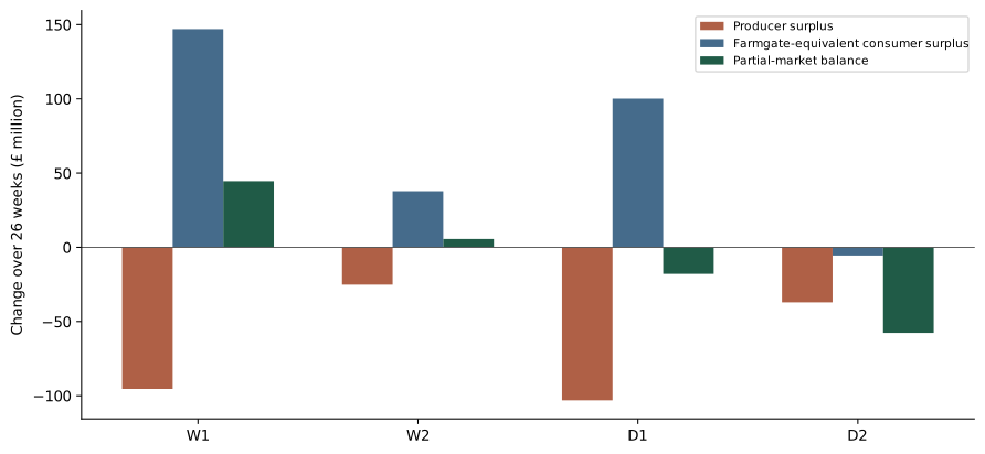
Without an imposed production loss, export displacement lowers the model price in both W cases. W1 produces a larger price fall and producer loss than W2. The positive partial-market balance in W1 follows from the consumer-surplus area in this particular trade closure and market-boundary approximation. It must not be interpreted as evidence that an outbreak improves national wellbeing: excluded intermediary margins, trading relationships, wider costs and non-market damage can change that conclusion.
With the 5% output shift, producer loss is £103.08m in D1 and £37.08m in D2. Recognition therefore improves this producer measure by £66.00m. Consumers move from a £100.15m gain to a £5.53m loss because price moves above baseline. The partial-market balance becomes more negative even as the producer position improves. A policy preference for continuity must therefore specify its distributional objectives and consider the omitted channels, rather than selecting the largest aggregate from this simplified market.
The no-recognition price-reversal threshold is 146/937 = 15.58% output reduction. With 80% recognition and a 10% restricted share it is 146 × 0.28 / 937 = 4.36%. The assumed D2 output reduction of 5% sits just above the latter threshold, explaining its small positive price change. These thresholds are algebraic properties of the chosen baseline and access formula, not estimates of likely production losses.
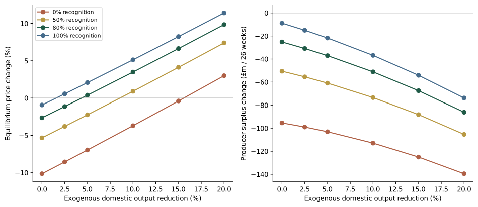
Table 10. Duration sensitivity for the D2 market assumptions
| Weeks | Producer £m | Consumer £m | Balance £m |
|---|---|---|---|
| 13 | -18.54 | -2.77 | -36.31 |
| 26 | -37.08 | -5.53 | -57.61 |
| 52 | -74.15 | -11.07 | -100.22 |
Changing duration scales annualised surplus changes while leaving the one-off £15m resource allowance unchanged. It does not simulate a sequence of prices, inventories or reopening dates. The elasticity sensitivity changes the degree of price adjustment and surplus response but does not move the zero-demand-shift price-reversal identity at the baseline price. Wider intervals should not be called more likely or less likely without a justified distribution for their inputs.
4.2 Farm-system losses and cash requirements
Table 11. Distinct illustrative enterprises; zero compensation in these defaults
| System | Gross loss £ | Finance £ | Net incl. finance £ | Peak borrowing £ |
|---|---|---|---|---|
| Breeder / weaner producer | £82,860 | £3,711 | £86,571 | £61,571 |
| Nursery / grower | £17,800 | £113 | £17,913 | £38,493 |
| Specialist finisher | £51,282 | £2,893 | £54,175 | £193,192 |
| Integrated farrow-to-finish | £256,137 | £19,170 | £275,307 | £541,967 |
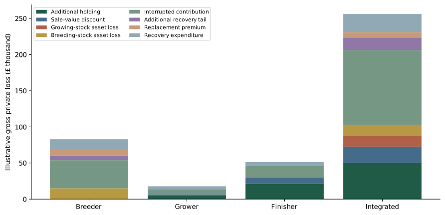
The breeder example combines interrupted contribution, breeding-stock loss, replacement premium and a later contribution shortfall. A reopening of slaughter capacity would not by itself remove these components. The grower example has a different sale value, holding cost, interruption length and external contribution from the finisher. The integrated example includes sow and growing-stock losses but uses one whole-chain contribution per external finished-pig sale. It does not sum the breeder’s £12 and finisher’s £20 as two independently lost revenues.
The normalised loss per annual marketed animal is also available in results.json, but it remains conditional on the selected scale, shock and contribution. It does not make unlike production stages economically equivalent. Representative comparisons would require matched farm accounts, enterprise size strata, contract terms and a common exposure design. The present examples answer how the accounting changes across systems.
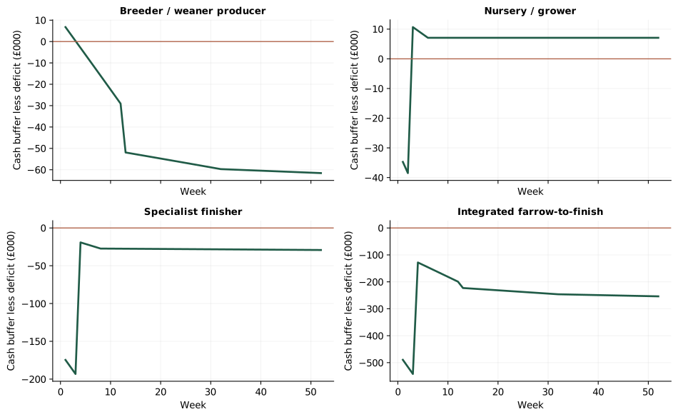
The finisher’s £51,282 gross economic loss accompanies a peak incremental borrowing requirement of £193,192 because a cohort’s normal sales receipts are postponed. Once surviving pigs are sold, those receipts re-enter the cash account. The remaining deficit reflects extra costs, lost contribution and finance. This illustrates why a payment or credit facility sized only to the eventual accounting loss may be too small at the point of maximum cash pressure.
For a breeder with no ready-to-market cohort in the selected template, missing output contribution accumulates and replacement outlay creates a later demand for cash. The integrated business experiences both mechanisms. All examples assume a zero normal net cash deviation after the disruption; they do not model retained future profits that might repay borrowing. Therefore a negative closing balance is not a solvency prediction and the horizon-end debt is not assumed written off.
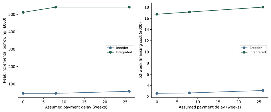
An earlier transfer can reduce financing without reducing the underlying resources lost. At unchanged compensation share, the economic loss before finance is the same for every payment delay; only the cash path and interest change. A delayed payment may leave the initial peak almost unchanged when that peak is caused by withheld sales, while increasing later interest. This distinction matters when comparing compensation administration, emergency lending and direct continuity measures.
4.3 Processing recovery is conditional on feasible capacity
Table 12. Recovery comparison at default assumptions
| Measure | Optimised additional capacity | Standard capacity |
|---|---|---|
| Discounted cost | £142,138 | £550,816 |
| Terminal backlog | 0 pigs | 3,000 pigs |
| Additional-capacity weeks | 6 | 0 |
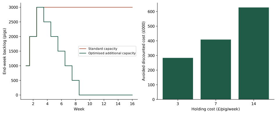
With arrivals equal to normal capacity, standard operations cannot reduce the backlog accumulated during the three-week closure. In the optimised example, an additional 500 pigs can be processed each week after reopening, so the 3,000-pig backlog is cleared through six weeks of extra capacity. The optimiser is evaluating the incremental expense of that capacity against holding and terminal costs. The result describes the economic value of an assumed capability, not proof that such spare capacity exists.
Table 13. Horizon and terminal-value checks at £7/pig/week holding cost
| Horizon weeks | Terminal £/pig | Optimal cost £ | Avoided cost £ | End backlog |
|---|---|---|---|---|
| 12 | 0 | £142,138 | £87,952 | 0 |
| 12 | 80 | £142,138 | £326,054 | 0 |
| 16 | 0 | £142,138 | £171,205 | 0 |
| 16 | 80 | £142,138 | £408,678 | 0 |
| 24 | 0 | £142,138 | £337,052 | 0 |
| 24 | 80 | £142,138 | £573,271 | 0 |
Sensitivity to the terminal value reveals the cost of pushing unresolved pigs beyond the planning window. A low penalty and short horizon can make delay appear cheaper; a larger penalty can favour earlier clearance. For the displayed baseline, the assumed extra capacity has time to clear the backlog within the tested windows. Extending the horizon should therefore be assessed alongside the standard-capacity counterfactual, whose unresolved stock continues to incur costs.
4.4 Compartment value is constrained by exposure, cost and recognition
The default expected annual avoided loss is £240,000: £100m × 30% × 50% × 80% × 2%. Discounted benefits over ten years are £2.00m against £13.32m in setup and recurring costs. NPV is £-11.32m and BCR 0.15. Holding other inputs fixed, break-even recognition is 333.6%, outside the feasible range. Better recognition alone cannot rescue this particular illustrative cost-and-exposure configuration.
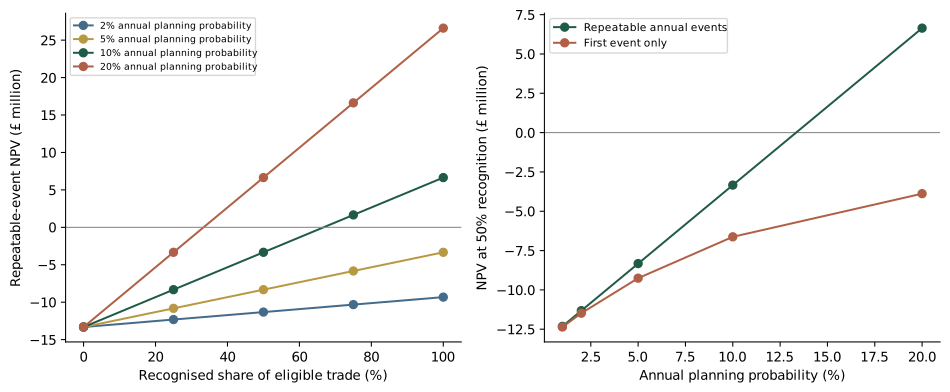
Table 14. Recognition delay and event-accounting sensitivities
| Annual probability | Delay years | Repeatable NPV £m | First-event NPV £m | Break-even recognition |
|---|---|---|---|---|
| 2% | 0 | -11.32 | -11.48 | 333.6% |
| 2% | 2 | -11.78 | -11.93 | 432.3% |
| 10% | 0 | -3.34 | -6.62 | 66.7% |
| 10% | 2 | -5.62 | -8.79 | 86.5% |
Higher assumed event frequency increases the value of protection, but the two event-accounting conventions diverge as frequency rises. The first-event model cannot accrue repeated event benefits after an initial opportunity. A recognition delay further reduces benefits while retaining operating costs. These structural choices should be resolved before presenting a single BCR. They are more consequential than displaying additional decimal places in an uncalibrated default.
5. Lessons from three MSc dissertations (2026)
The following assessment uses the supplied supervisor synthesis by Vosough Ahmadi (2026), not independently re-analysed dissertation datasets. The original dissertations are unpublished University of Edinburgh MSc work. Their contribution is to decision framing, mechanisms and research priorities. The programme, author and title are given in the references. Findings are not treated as peer-reviewed UK coefficients or as evidence that the present model has been validated.
5.1 Zang: the investment boundary changes the answer
Yifei Zang’s Ecological Economics dissertation assesses alternative ASF control strategies in China over 2018–2023. As summarised, a compartment scenario with 30% national slaughter coverage reports a BCR of 4.68 and effectiveness thresholds of 13.4% with consumer benefits and 20.4% without them. These are outputs of that dissertation’s model and its chosen benefit boundary, not observed programme returns. Parameter refinement is an explicit qualification in the synthesis.
The transferable lesson is to state whose benefits enter the numerator, what coverage means and which costs are required across the chain. The present UK illustration therefore distinguishes private loss avoidance from consumer surplus, separates participation, recognition and continuity, and shows an infeasible recognition threshold when costs exceed attainable benefits. The numerical resemblance of a 30% coverage example does not establish UK calibration; none of Zang’s reported BCR or effectiveness thresholds is used as a UK result.
5.2 Yang: output recovery and productive capacity are different
Shirong Yang’s Environmental Protection and Management dissertation examines Sichuan–Chengdu production, price patterns and organisational adaptation. The supervisor synthesis describes recovery in output or offtake alongside lower pig and sow inventories. This supports using several recovery indicators rather than reading slaughter recovery as complete restoration of the production system. Descriptive co-movement does not by itself identify the causal effect of consolidation, technology or any individual policy.
The corresponding UK design implication is practical: report breeding stock, marketed output, capacity use and business cash separately. A processing backlog programme should not be presented as a model of breeding-herd recovery. An integrated enterprise may restore sales by changing throughput or sourcing while still carrying replacement costs and financial stress. The current separate breeder and liquidity accounts make that distinction visible, but they do not estimate the organisational changes documented in Sichuan.
5.3 Zaidun: compensation and import dependence alter incidence
Dayang Ku Farah Ana Binti Zaidun’s Food Security dissertation combines Malaysian production and trade evidence with interviews, drawing on Asian experience during 2018–2024. The synthesis describes reduced domestic self-sufficiency, greater imports and concerns that compensation for official culling can leave earlier animal deaths outside payment. The interview base supplies context and hypotheses; it cannot establish population-wide effects or a causal relationship between a compensation rule and reporting behaviour.
The transferable questions concern eligibility, who lacks liquidity before payment, and whether recovered consumption is supplied domestically or through imports. The UK application consequently shows compensation as an explicit transfer, defaults it to zero, and tests payment delays separately from the rate. The market model allows imports to respond to price but does not estimate a long-run restructuring of domestic capacity. Those are distinct dimensions of resilience.
Table 15. From dissertation lesson to an auditable UK research question
| Study | Question carried forward | Evidence needed before a UK claim |
|---|---|---|
| Zang (2026) | Which participants and benefits make a compartment viable? | Verified UK participation, full-chain costs, access recognition and exposure |
| Yang (2026) | Has recovery restored capacity, throughput, or both? | Linked sow inventories, slaughter, enterprise survival and sourcing over time |
| Zaidun (2026) | Who is excluded from support, and when is cash required? | Eligibility records, payment dates, confidential farm accounts and representative interviews |
6. Discussion
6.1 Why the modules cannot be one national-loss number
The calculations answer different questions. Surplus changes describe price-and-quantity incidence in a stylised market. A private budget values the loss to one business. The weekly bridge describes the maximum funding gap relative to normal trade. A recovery programme values the marginal capacity decision. An investment appraisal values future avoided exposure. Summing those results would combine scales, time horizons and overlapping counterfactuals. A more elaborate visual presentation would not fix that accounting error.
A national impact estimate would require a consistent chain from controls and operational effects to quantities, prices, costs and transfers, with sector weights and uncertainty. The current release instead makes the location of each estimate and gap inspectable. It is suitable for comparing mechanisms, identifying data priorities and testing whether a proposed result depends on an implausible threshold. It should not be used to calculate compensation budgets by multiplying a single farm example by the national herd.
6.2 Interpreting indirect costs across the literature
Savioli et al. (2022) supplies the principal stakeholder-to-impact organising approach in Table 8. The priority mechanisms include transport logistics, demand response, preventing contact between wild boar and domestic pigs, and slaughter logistics. The current application quantifies selected economic pathways; it does not claim to have priced every identified measure. The transport and control allowances remain placeholders until a bottom-up UK inventory is costed.
Gren et al. (2024) reports approximately €28m in response costs for Sweden, with around 40% classified as indirect. That case demonstrates that local restrictions can affect activities outside livestock production. Its geographic setting, affected activities and accounting definitions differ from this UK scenario exercise. Neither the euro total nor the indirect-cost proportion is applied as a UK multiplier.
Helgesen and Barratt’s EPIC brief defines its indirect-cost window after disease freedom and models linked commodity price and revenue effects. In its medium scenario, a 20% national herd cull is associated with a British pork-producer revenue loss of £53.50m. Revenue is not surplus, and post-freedom persistence is not the same period as the constant disruption used here. The comparison identifies an omitted recovery channel; it does not provide a second number to add to Table 9.
Shakil et al. (2025) illustrates why a vertically connected livestock model can represent incidence beyond the farm gate. A UK extension would need stage-specific prices and processing costs, product conversion, substitution and trade destinations. The present single-market approximation does not implement that published vertical model. Making the distinction explicit prevents the literature review from suggesting analytical capabilities absent from the code.
6.3 Epidemiological evidence and economic uncertainty
Shaw, McLure and Glass (2024) examines how ASF model assumptions and structure affect conclusions. Fay et al. (2025) examines the importance of seasonal timing in host–pathogen dynamics. These open research contributions support treating duration and production effects as uncertain and potentially dependent. They do not justify selecting one UK loss percentage, nor does citation supply current UK validation. This paper models economic consequences conditional on specified disruptions and contains no simulation of infection or transmission.
The implication for future economic work is to preserve provenance at any model interface: record the scenario definition, geographic coverage, time resolution and uncertainty of externally supplied consequences before translating them into economic inputs. Current authorised data, independent validation and jurisdiction-specific policy interpretation would be required for an operational forecast. Historical haulage evidence in Porphyre et al. (2020) remains a reason to examine shared-service disruption, rather than a current map of vulnerable routes.
6.4 Distribution, liquidity and investment feasibility
A reduction in aggregate producer loss can coexist with severe losses in a subset of breeders or export-dependent finishers. An integrated chain may retain coordination advantages while requiring much more liquidity in absolute terms. Smaller independent businesses may face higher fixed compliance cost per unit and weaker access to credit. These distributional hypotheses are economically plausible but are not quantified by comparing differently sized default farms.
The compartment calculation also separates feasibility from financial performance. Even a positive conditional NPV would not establish access recognition, acceptable participation terms or implementation capacity. Conversely, a negative private NPV does not rule out a public case with additional verified public benefits. That broader case would need its own resource, transfer and distributional boundary, consistent with the Green Book’s emphasis on more than a single BCR (HM Treasury, 2026b).
6.5 Principal limitations
Table 16. Limitations that can change interpretation
| Limitation | Consequence | Required improvement |
|---|---|---|
| No empirical elasticity or disruption calibration | Magnitude and sometimes policy ranking depend on assumptions | Estimate or justify ranges with UK evidence |
| Homogeneous pigmeat and complete price transmission | Household benefit and exporter incidence can be misrepresented | Product, stage and destination differentiation |
| Constant shock interval | No reopening path, inventory dynamics or endogenous recovery | Observed schedules and a dynamic economic model |
| Farm templates not sampled | No prevalence or national extrapolation | Representative enterprise accounts and weights |
| Simplified cash bridge | No full debt service, tax, normal retained cash or insolvency model | Bankable weekly farm budgets |
| Assumed feasible processing capacity | Optimiser may select unavailable actions | Verified operational and welfare constraints |
| Private compartment boundary | Public benefits and distribution absent | Separate social and participant appraisals |
| Uncertainty grids without probabilities | No forecast likelihood, confidence interval or expected national loss | Justified joint distributions and external validation |
7. Implications and recommendations
Preparedness should begin with a shared definition of the decision and its counterfactual. For trade, that means recognition by product and destination rather than a binary promise of regionalisation. For support, it means separating permanent economic loss from a temporary withheld receipt. For recovery, it means checking which capacity and housing constraints are actually binding. For investment, it means resolving whose exposure and costs are included before calculating a BCR.
Table 17. Priority actions, evidence owners and decision outputs
| Priority action | Evidence partners | Concrete decision output |
|---|---|---|
| Reconcile the pigmeat baseline and product scope | Official statisticians, AHDB and trade analysts | One documented balance with offal, processed products and vintages reconciled |
| Calibrate four enterprise budgets | Breeders, growers, finishers, integrated businesses and accountants | Anonymised stock-flow budgets, contribution margins and cash schedules |
| Build the indirect-cost register from the bottom up | Hauliers, processors, producers, authorities and affected rural businesses | Cost items with counterfactuals, dates, quantities and overlap tags |
| Prepare recognition-specific economic cases | Competent authorities and industry market-access teams | Destination/product access assumptions with evidence and uncertainty |
| Check real recovery constraints | Processors, transport providers and welfare specialists | Feasible action set and independently checked capacity costs |
| Test support timing and coverage | Industry, lenders and payment administrators | Peak funding and residual loss by enterprise and eligibility case |
| Stage-gate compartment appraisal | Participants, auditors, authorities and trading partners | Verified scope, cost quotes, recognition milestones and distributional assessment |
| Commission independent model review | Agricultural economists and end users | Calibration report, reproducibility checks and documented limitations |
The first analytical investment should be in data that can change a decision: current stage-specific contribution margins, delayed-sale schedules, full-chain continuity costs and evidenced recognition assumptions. More detailed numerical optimisation cannot compensate for a missing cost item or a mis-specified counterfactual. The existing modules can be re-run with better economic evidence without treating the illustrative defaults as authoritative.
8. Conclusions
ASF economic preparedness requires several connected accounts rather than one headline damage figure. The illustrative market results show how recognition can reduce producer loss while changing consumer incidence; farm results show why liquidity can exceed economic loss; processing results show the conditional value of extra capacity; and the investment analysis shows when recognition cannot overcome an unfavourable cost-and-exposure structure. These are economic mechanisms and thresholds, not predictions of the size or timing of a UK event.
The contribution of this release is an explicit evidence hierarchy, four enterprise boundaries, a genuine weekly incremental cash path, an indirect-cost coverage register and reproducible scenario results. The next step toward a decision-grade appraisal is UK calibration and independent review, followed by a coherent integrated accounting framework where broader effects are required. The present analysis should be used to formulate and scrutinise those questions.
Acknowledgements, authorship and disclosure
Prepared for the Syntera economic observatories under the authorship of Dr Bouda Vosough Ahmadi. The analysis acknowledges the published contributions of Giulia Savioli, Violeta Muñoz, Fabrizio Rosso and Manon Schuppers; Thibaud Porphyre, B. M. de C. Bronsvoort, George J. Gunn and Carla Correia-Gomes; C. Shaw, A. McLure and K. Glass; R. Fay, M. Gamelon and E. Baubet; I.-M. Gren, H. Andersson and L. Jonasson; Irmelin Helgesen and Alyson Barratt; and Golam Saroare Shakil, Dustin L. Pendell, Jonathan Rushton and Thomas L. Marsh. Full attribution appears in the reference list.
Yifei Zang, Shirong Yang and Dayang Ku Farah Ana Binti Zaidun are acknowledged for the 2026 MSc work described in the supervisor synthesis. Public evidence and guidance are credited to Defra, AHDB, EPIC Scotland, WOAH and HM Treasury. These acknowledgements recognise the sources used; they do not imply that the named researchers or organisations reviewed, contributed to, approved or endorsed this implementation. Original dissertation files, confidential movement data and private proposal materials are not redistributed.
Bouda Vosough Ahmadi is a co-author of Savioli et al. (2022) and provided the synthesis used for the dissertation discussion. Those relationships are disclosed to make the basis of selection and interpretation clear. AI-assisted drafting, coding and consistency checks were used in preparing this revision. No independent peer review or empirical validation of the illustrative assumptions is claimed. Responsibility for any public or operational use requires substantive expert review.
Disclaimer
Independent, exploratory working paper, version 3.0.0, evidence checked 23 September 2026. Outputs are conditional on stated assumptions and are not official estimates, epidemiological forecasts, movement permissions, legal advice, compensation entitlements or investment recommendations. This work is not commissioned, validated or endorsed by AHDB, Defra, APHA, the University of Edinburgh, EPIC, FAO, WOAH or GF-TADs. UK economic aggregates do not replace jurisdiction-specific policy interpretation. Errors or unresolved data differences should be corrected before decision use.
References
Defra (2026a). Agriculture in the United Kingdom 2025, Chapter 8: Livestock. Updated 3 September 2026. Source ↗
Defra (2026b). African and classical swine fever disease control strategy for Great Britain. Updated 21 May 2026. Source ↗
AHDB (2026a). Q1 2026 pork cost of production. 11 May 2026. Source ↗
AHDB (2026b). UK pork outlook 2026: June production update. 22 June 2026. Source ↗
Savioli, G., Vosough Ahmadi, B., Muñoz, V., Rosso, F. and Schuppers, M. (2022). A methodology to assess indirect economic impacts of animal disease outbreaks: A case of hypothetical African swine fever outbreak in Switzerland. Transboundary and Emerging Diseases, 69, e1768–e1786. Source ↗
Porphyre, T., Bronsvoort, B.M. de C., Gunn, G.J. and Correia-Gomes, C. (2020). Multilayer network analysis unravels haulage vehicles as a hidden threat to the British swine industry. Transboundary and Emerging Diseases, 67(3), 1231–1246. Source ↗
Shaw, C., McLure, A. and Glass, K. (2024). African swine fever in wild boar: investigating model assumptions and structure. Royal Society Open Science, 11, 231319. Source ↗
Fay, R., Gamelon, M., Baubet, E. and Porphyre, T. (2025). The time of infection matters: seasonal interplay between host and pathogen drives epidemic dynamics. Oikos, 2025, e10750. Published online 16 December 2024. Source ↗
Gren, I.-M., Andersson, H. and Jonasson, L. (2024). Benefits and costs of measures to tackle the outbreak of African swine fever in Sweden. Preventive Veterinary Medicine, 233, 106353. Source ↗
Helgesen, I. and Barratt, A. (n.d.). Policy brief: Indirect cost of ASF. EPIC Scotland. Accessed 23 September 2026. Source ↗
Shakil, G.S., Pendell, D.L., Rushton, J. and Marsh, T.L. (2025). Economic Burden of Livestock Diseases: A Vertically Integrated Partial Equilibrium Livestock Model. Agricultural Economics, e70062. Source ↗
World Organisation for Animal Health (WOAH) (2021). Guidelines on compartmentalisation for African swine fever. Paris: WOAH. Source ↗
HM Treasury (2026a). The Green Book: Central Government Guidance on Appraisal and Evaluation. Source ↗
HM Treasury (2026b). Green Book Review 2025: One year on. 30 June 2026. Source ↗
Zang, Y. (2026). From Blanket Restriction to Compartmentalisation: An Economic Assessment of Alternative African Swine Fever Control Strategies in China. Unpublished MSc dissertation, Ecological Economics, University of Edinburgh. Consulted through Vosough Ahmadi (2026).
Yang, S. (2026). Resilience of the Sichuan–Chengdu Pork Supply Chain Following African Swine Fever: Production, Price Dynamics and Organisational Adaptation. Unpublished MSc dissertation, Environmental Protection and Management, University of Edinburgh. Consulted through Vosough Ahmadi (2026).
Zaidun, Dayang Ku Farah Ana Binti (2026). The Impact of African Swine Fever on Pork Production, Trade and Self-Sufficiency in Malaysia: A Mixed-Methods Analysis Informed by Evidence from Asia, 2018–2024. Unpublished MSc dissertation, Food Security, University of Edinburgh. Consulted through Vosough Ahmadi (2026).
Vosough Ahmadi, B. (2026). ASF control and recovery lessons from China and Malaysia: policy synthesis for FAO, WOAH, GF-TADs and national authorities. Unpublished supervisor synthesis supplied for this analysis, 22 September 2026.
All public web references were consulted for this revision on 23 September 2026. Unpublished dissertation claims are attributed through the supplied supervisor synthesis; the original theses were not independently reviewed. Official releases retain their observation period, which differs from publication and access dates.
Appendix A. Reproduction, parameter audit and numerical conventions
The downloadable bundle contains models.js (market and recovery), enterprise.js (four enterprise accounts and investment), run_publication.js, test-models.js, results.json and CSV sensitivity tables. From the extracted bundle, run “node test-models.js” and then “node run_publication.js”. These commands require Node.js and no external JavaScript packages. The runner regenerates numerical outputs under dist/publications/asf-economics-2026-09/. Figure and document generation additionally uses Python with NumPy, Matplotlib and ReportLab; build_publication.py is included. Neither script downloads data or third-party papers.
The source of truth is the versioned model code and input objects stored in results.json. Tables are formatted from that output and figures are drawn from the same arrays. Rounding occurs only for display except in the documented 50-head processing grid and whole-week cash schedule. CSV values preserve numerical precision. Sensitivity ranges are selected exploration values. They are not confidence limits and are not sampled from inferred distributions.
Table A1. Parameter groups not empirically calibrated in this release
| Module | Assumed parameters | Units / convention |
|---|---|---|
| Market | Duration, output/demand shifts, blockage, recognition, restricted share, all elasticities, control/logistics | Weeks, percentages, local elasticities, one-off £m |
| Farm | Stock, losses, contribution, holding, discount, recovery, compensation, timing, cash buffer and interest | Head, £/head, days, weeks and annual percentage |
| Farm derived proxy | Finisher sale value = 91 × 2.04 | £185.64/head; combines annual statistical averages |
| Processing | Arrivals, capacity, restriction, extra capacity, all cost rates, terminal value and horizon | Head/week, £/head/week, £/head and weeks |
| Investment | Exposure, coverage, recognition, continuity, event probability, costs, life and delay | Real £m, percentages, years; probabilities illustrative |
The no-shock market baseline clears at p₀ by construction, not by an out-of-sample prediction. Local linear schedules are clamped at zero and can be unrealistic far from calibration. No price, output or cost series is forecast beyond the selected counterfactual. Compensation transfers are omitted from the partial-market balance; adding them as national losses would violate the chosen resource boundary. Where an official programme has administration costs, those resources require a separate evidenced entry.
Version 3 replaces combined grower/finisher treatment with four enterprise templates; values the integrated external contribution once; adds weekly liquidity, compensation-delay sensitivities and recognition-delay and first-event investment variants; corrects inverse-supply integration for elasticities above one; and generates the publication from the same numerical engine. Earlier static summaries and their figures are superseded by this version. Numerical verification is recorded by the accompanying test script, not represented as external model validation.